Mesoscale Research Current Product Development

Figure 1: An image loop created from McIDAS AREA files of a three-color dust product. This example shows a large dust cloud over Libya and dust being drawn into a low pressure center over the Mediterranean . Dust is pinkish-red, thicker clouds are yellowish-green, and cloud-free areas are light blue. Note that occasional flashes of contrasting colors are due to the way McIDAS deals with too many colors. A solution for that problem is currently being tested. [Click on the image to start the loop.]

The 3-color product generation routine used for the dust product loop has now been improved, to eliminate a color-shift problem. The improvement required a reduction from 256 colors to 128 colors, to compensate for the occasional color shifts that McIDAS imposes on all 256-color images. That color shift resulted in strongly-contrasting colors appearing in the 3-color image, especially associated with the color tables needed for these three-color products. The problem was more noticeable when an image loop was created from the 3-color product. By reducing to 128 colors, and each color now representing two 8-bit count values, the occasional color shifts are no longer a problem. See the attached two figures, utilizing MSG full-disk imagery, for examples of the 256 and 128-color versions, respectively. Viewers will be hard pressed to see differences in the images unless they are directly compared. The more noticeable change is in the colored bar at the bottom of the image, with slightly larger color bins for the reduced-color version. (D. Hillger)

Figure 1a: A 3-color McIDAS AREA created from three separate (red, green, and blue) McIDAS AREA files. This example shows the MSG “natural” color product created from MSG bands 3, 2, and 1, respectively. This version uses all 256 possible colors allowed on 8-bit displays.

Figure 1b: Same as Figure 1a, except utilizing only 128 different colors. Note the elimination of the narrowest color bins in the color bar at the bottom of the image. There are also subtle differences in the image that can be seen if the user were to directly compare the two images.

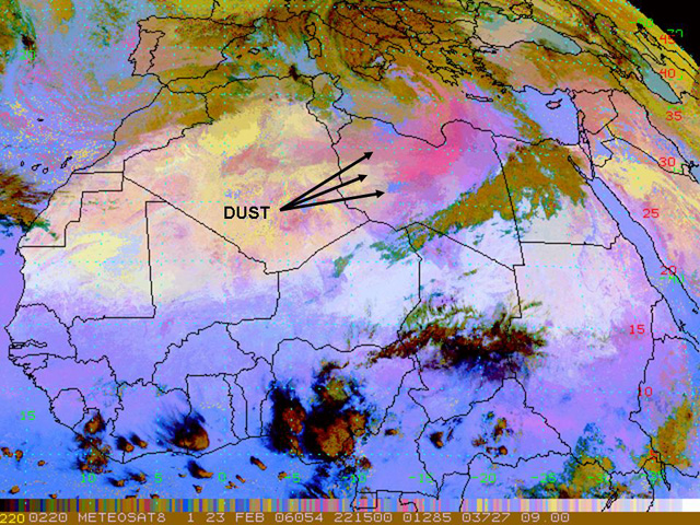
Two other examples of the 3-color dust product from real-time MSG (Meteosat Second Generation) imagery have been captured. The dust product uses software developed to create McIDAS-formatted AREA files from three images assigned as the red, green, and blue components. In this case the product is a second-order combination, via band differencing, of three MSG IR bands (8.7 µm, 10.8 µm, and 12.0 µm). These examples utilize software that was improved to eliminate color-flickering associated with too many colors, and a second problem caused by saturated pixels in the inputs to the 3-color algorithm. The first loop is a good example of a widespread dust outbreak associated with a cold front moving south across most of northern Africa . The second loop is an example of dust being drawn into a low pressure center tracking to the east, ingesting dust from off of West Africa . Dust is pinkish-red, thicker clouds are yellowish-green, and cloud-free areas area light blue. This dust product is being developed as part of GOES-R Risk Reduction activities. (D. Hillger)

Figure 1a: An image loop created from McIDAS AREA files of a thee-color dust product. This example shows a widespread dust outbreak associated with a cold front moving south across most of northern Africa . Dust is pinkish-red, thicker clouds are yellowish-green, and cloud-free areas are light blue. [Click on the image to start the loop.]

Figure 1b: As in Figure 1a, but this example shows a low pressure center tracking to the east, ingesting dust from off of West Africa . [Click on the image to start the loop.]

Synthetic GOESR-ABI images from the simulation of the 8 May 2003 severe weather case have been used to develop new products. Specifically, preliminary development of channel differencing between 6.185 µm, 10.35 µm, and 12.3 µm has begun. (L. Grasso, D. Lindsey, and B. Connell)

A web page was developed to display the mesoscale convective system (MCS) index which was developed by Israel Jirak of Colorado State University. (H. Gosden, D. Lindsey, I. Jirak) (H. Gosden)

Processing of the large sector U.S. climatologies continues.  Products completed include monthly large sector composites for November and December 2005.  Processing is behind schedule, but should be caught up by next quarter. (C. Combs)

Processing of wind regime products continues.  Monthly wind regime composites from both channel 1 and channel 4 for October, November and December 2005 have been completed.  Combined monthly products have also been completed for these months and channels.  (C. Combs)

Hired new student hourly to replace departing hourly for cloud composite work.  Training is in progress. (C. Combs)

Work on the new cloud climatology project with Eureka , CA continues. Data processing for the Eureka sector for July 1999-2005 is complete and August 1999-2005 nearly complete. Three time series of cloud composites(low, high and all) have been derived from the 10 µm channel for July 1999-2005.   Examples from the results have been shared with the Eureka , CA  National Weather Service (NWS) office (figures 1 and 2). (C. Combs)

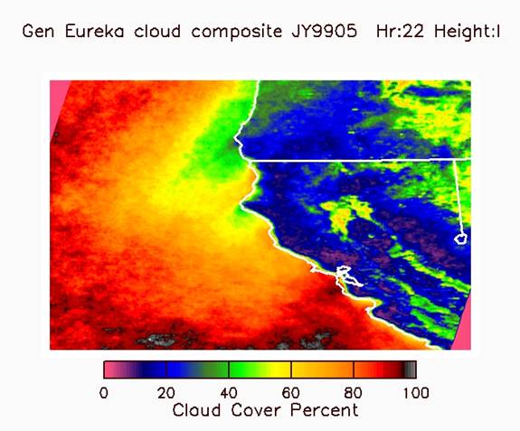
Figure 1: Low cloud composite for July 1999-2005 for 2200 UTC (3 pm local)

Figure 2: Low cloud composite for July 1999-2005 for 1000 UTC (3 am local)

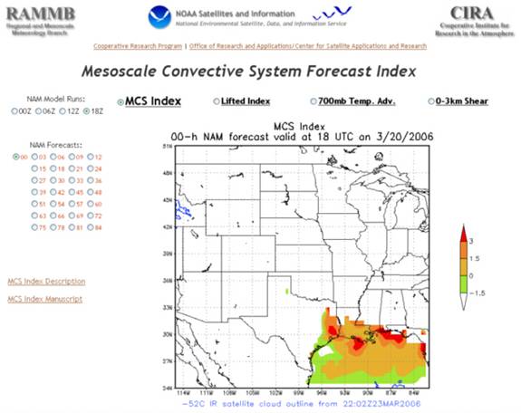
An experimental Mesoscale Convective System (MCS) Index has been developed in collaboration with Israel Jirak (Dept. of Atmos. Sci., CSU). This automated product predicts areas supportive of MCS formation and organization. It utilizes NAM model output, and GOES IR satellite data is currently used on the webpage and will be used for validating the product. The webpage is: http://rammb.cira.colostate.edu/projects/mcsindex/mcsindex.asp . The Figure below shows an example MCS Index forecast. (D. Lindsey)

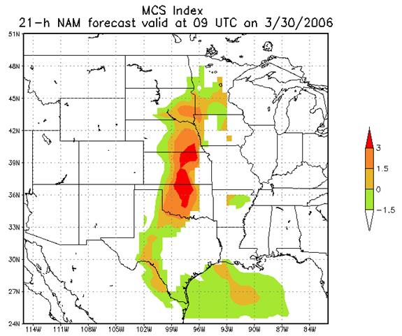
MCS Index forecast from 12Z on 29 March 2006, valid at 09Z on 30 March 2006.

Work is nearly complete on an ice cloud effective radius retrieval product. This uses the GOES 3.9 µm and 10.7 µm channels, and is valid for optically thick clouds composed of ice crystals, which includes thunderstorm tops. Results from Lindsey et al. (2006, mentioned below) show a correlation between small thunderstorm top ice crystal size and updraft strength, so a second product will be created taking advantage of this relationship. (D. Lindsey)

Employing a method originally developed for use with tropical cyclones, a wind retrieval technique using vertical temperature profiles derived from radiances from the Advanced Microwave Sounding Unit (AMSU) is being developed for the polar regions. With a boundary condition given by a 100-hPa height field from the Global Forecast System (GFS) analysis, the temperature profiles are used in the downward integration of the hydrostatic equation to compute height as a function of pressure. A balance condition is then applied to compute the stream function, from which the u- and v-components of the non-divergent wind can be evaluated.

As a first step, geostrophic balance was assumed in the derivation of the wind field. Fig. 1 shows the bias and rmse of the geostrophic wind speed derived using the AMSU technique when compared to the actual wind speed measured by radiosondes launched from various Arctic stations during a portion of December 2004. The bias and rmse are minimized at the levels where the wind is approximately in geostrophic balance. The two areas where this occurs are in the middle troposphere and in the stratosphere. Near the surface and near the jet level, the geostrophic wind is not as good an approximation, and the bias and rmse are increased. These two areas are also regions of the atmosphere where the retrieval of temperature by satellite is less accurate. For the free atmosphere overall, the bias is under 3 m s -1 and the rmse is under 7 m s -1 .

The next step was to solve the linear balance equation to retrieve the wind field. Fig.1 also shows the statistics for the comparison between the linear balance winds and the winds measured by radiosonde. The use of the linear balance results in typical improvements in the bias and rmse of around 0.5 ms -1 over the geostrophic balance.

In the future, the nonlinear balance equation will be solved; this should further increase the accuracy of the retrieved wind field. (J. Dostalek and M. DeMaria)

Figure 1. Bias (solid) and rmse (dashed) of retrieved winds as compared to winds measured from radiosonde. The black lines are for the geostrophic winds and the red lines are for the linear balance winds. The numbers along the vertical axis on the right-hand side are the number of comparisons for each level.

Return to the current RAMM Branch Quarterly Report